Six Degrees of NBA Players - A BFS Approach
I. Introduction
Think of your favorite celebrity that has been in a movie. It is almost guranteed that through a web of mutual costars, there will always be a path that leads to Kevin Bacon. What's even more wild, is that you will probably find a connection that only needs 6 or less costars. Don't believe me, you can try it yourself by visiting The Oracle of Bacon. We'll go over the math in a bit, but I just wanted to introduce this website as a bit of a primer for what we are going to discuss, for it was this project that prompted the idea of creating a similar application, but using only NBA Players.
With this context, I created NBA Teams Apart (NBATA). NBATA is a simple web application in which you can select any two basketball players in professional history dating all the way back to 1947, and you will find a connection between them through shared teammates. If you want to try it yourself, you can visit NBATeamsApart.com.
II. Only Six Degrees, How?
It seems a bit remarkable that if you pick any two players in basketball history, that you will be able to find a chain of teammates that is pretty much always going to be less than 6 players. But why?
The answer to this is related to Graph Theory. Graph theory is a methematical branch that deals with the way objects are related to each other. I'm not going to go into a ton of depth into this because it's a bit outside of the scope of this simple blog post, so instead we'll go through a quick math exercise.
Four years ago, there was a Reddit post that indicated that there have been 5,018 players that have played in the NBA. To keep numbers simple, let's say that there are now 6,000 players in the league since the time this post was made. A big jump but we like round numbers over here.
\( T_p = 6000 \)
I feel like for some people, seeing this number is already making the claim that we can make a connection between two basketball players, a bit more believable. Let's continue. Now we're going to make the assumption that each player has 14 different teammates at a time. This is to assume that each NBA roster has 15 players.
\( N_p = 14 \)
Now, it's reasonable to assume that not every team was created only through draft picks since the inception of the team. So, to go take into account teams being traded, signed, and waived. Let's say that 7 players from each team have also been a part of a different team.
\( N_t = 7 \)
This means that those 7 teammates that came from a different team have a connection with 14 different players. Putting the pieces together, that means that any single player on a team \( P_c \) already has a network of 91 unique players.
\( P_c = (N_p * N_t) - N_t \)
\( P_c = (14 * 7) - 7 \)
\( P_c = 91 \)
So with just one player and one connection, we get 91. What happens if we want to expand this into two connections. Well to keep it simple, we can just square the number we calculated and get \( P_{c2} = 8,281 \). 8,281 players alraedy puts us above all NBA players in history. Of course the numbers don't explode that quickly when it comes to our example. There is a bit of overlap between players and teams and I don't think I need to clarify this but not all 6,000 players were active at the same time. The point of this example was to show how quickly numbers can blow up.
This example has some backing though. Facebook did an in-depth analysis to determine what the average distance between users on Facebook was and the answer was 4.7. A shockingly low number. If you want to read the entire paper, you can find it here, The Anatomy of the Facebook Social Graph
III. A Breadth First Search Approach
The math is great and all but how exactly do we implement an algorithm to filter through every player, every team, and every connection to ensure that not only do we get the correct answer, but we don't run a million calculations every single time. Enter Breadth-First Search (BFS).
.png)
BFS is an algorithm that traverses nodes in a graph by exploring every neighbor at the current level before moving on to the next. This is different from Depth-First Search (DFS), which follows a path as far as it can before backtracking. While both algorithms have their place, if the goal is to find the shortest path between two nodes, BFS is typically the better choice. Because it explores all nodes at one “layer” before moving deeper, the first time you reach a node you can be confident that you’ve found the shortest path to it. With DFS, you would need to explore every possible path to guarantee the shortest one.
Let's use an example with NBA context.
Let's say we want to find the relationship between Stephen Curry (Player A) and Anthony Edwards (Player B).
The first thing we need to do is get a list of all the teams that Steph Curry has played on in his career.
| Team ID | Team Label | Season |
|---|---|---|
| GSW10 | Golden State Warriors | 2009-10 |
| GSW11 | Golden State Warriors | 2010-11 |
| GSW12 | Golden State Warriors | 2011-12 |
| … | … | … |
| GSW25 | Golden State Warriors | 2024-25 |
| Player ID | Player Label | Team ID |
|---|---|---|
| azubuke01 | Kelenna Azubuike | GSW10 |
| bellra01 | Raja Bell | GSW10 |
| ellismo01 | Monta Ellis | GSW10 |
| … | … | … |
| spencpa01 | Pat Spencer | GSW25 |
\[ \text{Seen}_{\text{Teams}} = \{ \text{GSW}_{10}, \text{GSW}_{11}, \text{GSW}_{12}, \ldots, \text{GSW}_{25} \} \]
\[ \text{Seen}_{\text{Players}} = \{ \text{azubuke01}, \text{bellra01}, \text{ellismo01}, \ldots, \text{spencpa01} \} \]
I also mentioned a queue earlier. For our first iteration, our queue is going to look the same as the SeenPlayers set. That's because our queue is going to have every player from every team that Player A has played with.
\[ \text{queue} = \{ \text{azubuke01}, \text{bellra01}, \text{ellismo01}, \ldots, \text{spencpa01} \} \]
\[ \text{res} = 1\]
The res simply represents which iteration or "step" we are on.
From here, because we know who Player B is, we simply iterate through all players until we get a match.
In this case, we are iterating through all of the names in the queue until we find Anthony Edwards (edwaran01).
This is where things get interesting! Because we know that Anthony Edwards and Steph Curry never played together,
Anthony Edwards is not going to be in the queue.
So what we do now, is we repeat that same process of iterating through each teammate that a player has had in their career,
with every single player in the queue. Steph Curry alone has played with 100+ different teammates.
Imagine how many players are going to be in our SeenPlayers set once we iterate through all of those players
and figure out how many teammates all of those players have played with, combined.
Doing an example like this shows us just how quickly these numbers can explode.
It also takes a bit of the magic away from it but that's okay!
If you're curious to see what the link between Steph Curry and Anthony Edwards is, here's what my algorithm calculated.
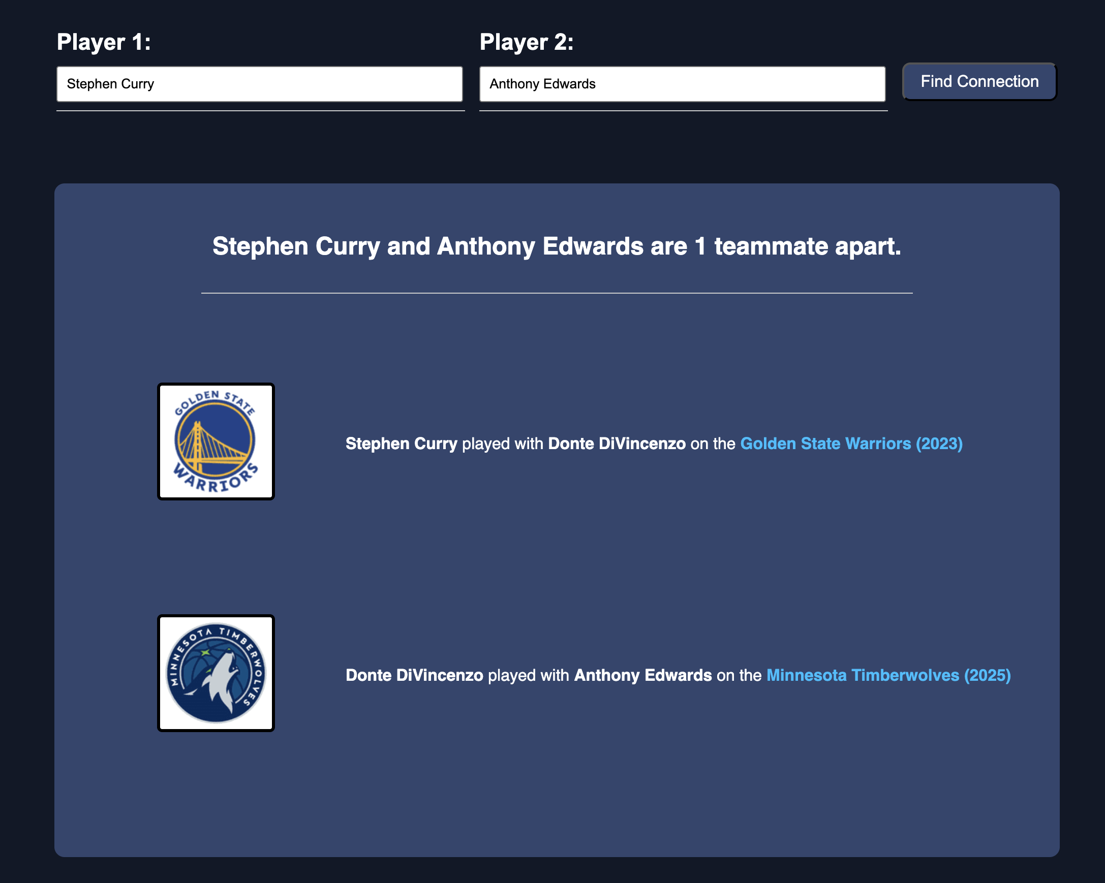
Looking at it from a tree perspective, it sort of looks like this
IV. Thoughts
I wanted to pop by and make a few notes. First of all, even though our algorithm said that the shortest bath between Curry and Ant is through the use of Donte, that does not mean that it's the only valid path. To keep things optimized, the algorithm exits out of the iteration and returns the chain the moment it finds its first connection. As mentioned, this is because BFS will always return the shortest path between two objects. There is no need to keep iterating through names because we know for a fact that we alraedy have the shortest path. For example, we know Kyle Anderson also played for the Timberwolves alongside Anthony Edwards and he also played on the Warriors. Curry -> Anderson -> Edwards is a valid connection, but because it's the same length as the connection with Donte, it doesn't really matter.