Vectors

A Simple Line

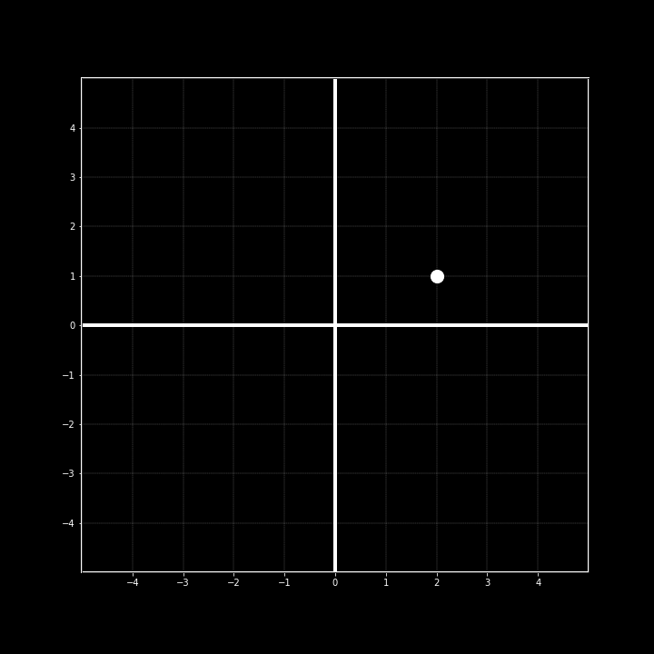
Before we begin to even talk about matrices and linear algebra, it's important to start off with the basics and build our way up. Having a fundamental understanding of how the systems at play work will make concepts later on a lot easier to grasp. In terms of linear algebra, the simplest place to start is with vectors. To begin, let's imagine we have some arbitrary point on a simple graph. For our example, let's have at the coordinate ( 2 , 1 )

From here, we can imagine a line that starts at the origin ( 0 , 0 ), connecting to this arbitrary point.

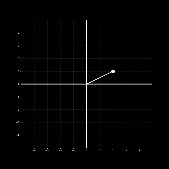
At this point you may be asking yourself, "Okay, so what's the big deal? This is just a simple line." and at this point, you would be correct. What we have shown here is nothing but an ordinary line. We can figure out what the slope of it is pretty easily (0.5) as well as the y-intercept (0). Beyond this, there is not much more we can extrapolate.

Next, I am going to replace the line with a vector.

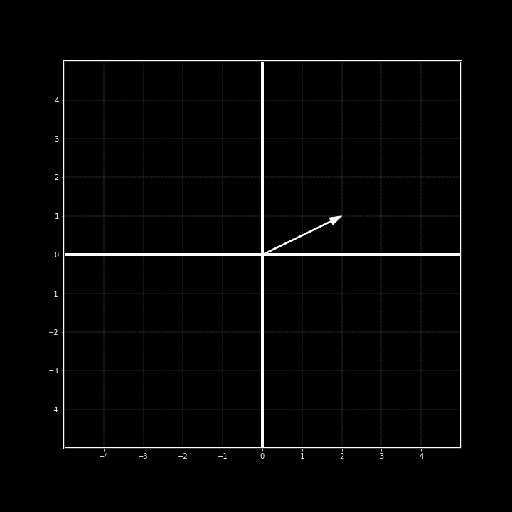
At first glance, it looks like the line was replaced with an arrow, and in a way that's true. There are two important attributes that quantifies this "arrow" as a vector: direction and magnitude. Let's break each one down.

Magnitude

The easiest way to think about magnitude is by imagining that magnitude is essentially the intensity or length of the vector. To find the magnitude we can easily use the coordinate of the vector point and plug the numbers into the following:

\[\sqrt{(x_2 - x_1)^2 + (y_2 - y_1)^2}\]

In our case, our vector starts at ( 0 , 0 ) and ends at ( 2 , 1 ). This leads us with a magnitude of \(\sqrt{5}\).

This equation can be derived from the Pythagorean and is relatively straight forward. Let's go ahead and add another vector to our graph and try this equation again.

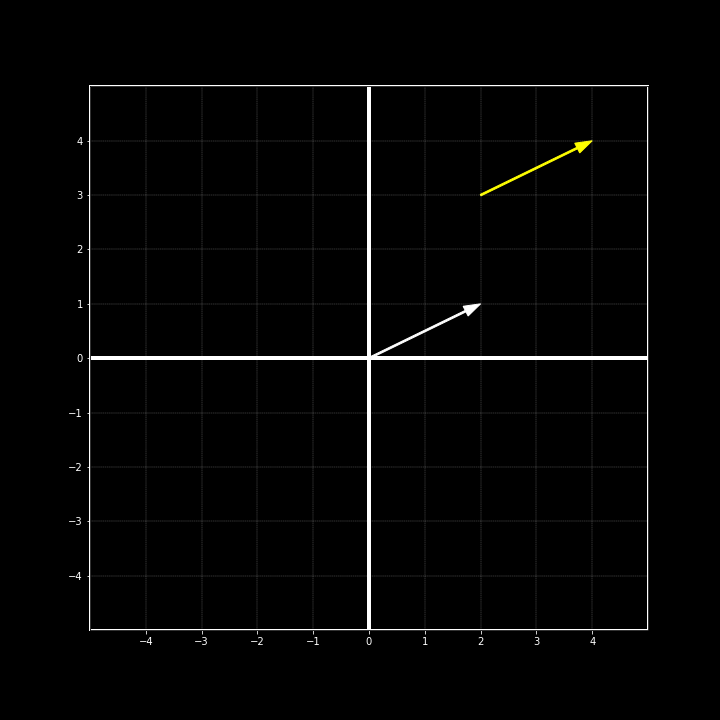
Using the equation from earlier, we can plug in the new values from the new vector and get the following:

\[\sqrt{(x_2 - x_1)^2 + (y_2 - y_1)^2}\] \[\sqrt{(4 - 2)^2 + (4 - 3)^2}\] \[\sqrt{5}\]

We find that we also get \(\sqrt{5}\) as our answer, even though these vectors are not located at the same spot. It's for this reason that it always best to try to have the arrays begin at the origin. It makes calculations a lot easier. We just discovered that both of these arrays have the same magnitude, so does that mean that these two arrays are the same? Maybe. It is important to notice that there are two characteristics that apply to each array. We have simply looked at the magnitude, it is now time to look at direction.

Direction

Finding the direction of an array simply means finding the angle of that array. The typical reference that is used to calculate this angle is the x-axis. Let's use the same array as before. This time we'll be a bit more proper with our notation.

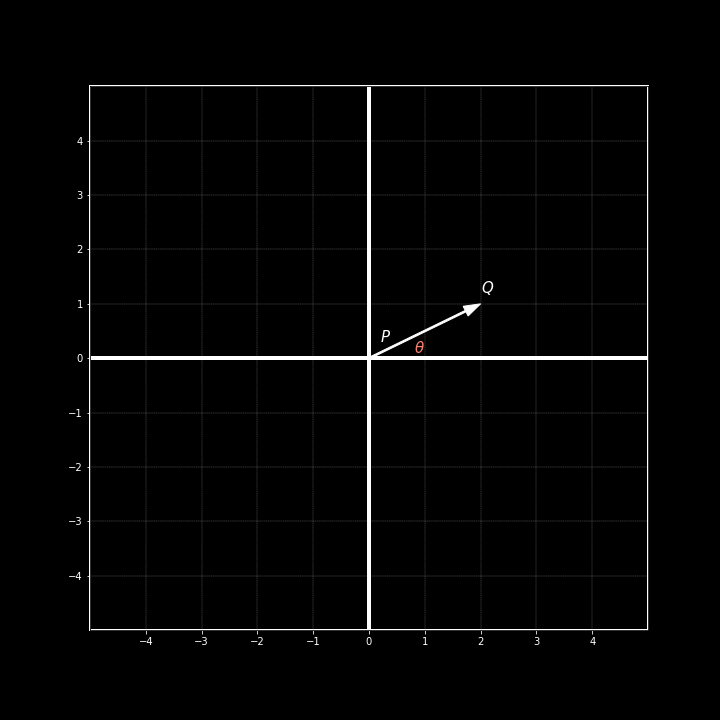
As we can see, we have introduced a new \(\theta\) value in addition to properly annotating the two ends of our array. The \(\theta\) value represents the angle that we are trying to uncover. If we take a closer look at the array and x-axis we might begin to notice something.

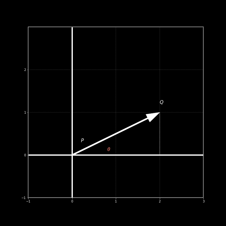
It looks just like a triangle! Thinking back to trigonometry, we can see that a simple tan() operation can be used here to find the missing angle. All we would need to do is find the length of the adjacent and opposite side with the respect to the angle. Luckily, we know how to do that.

\[tan\theta = \frac{adjacent}{hypotenuse} = \frac{y_2 - y_1}{x_2 - x_1}\]
\[tan\theta = \frac{1 - 0}{2 - 0}\] \[tan\theta = \frac{1}{2}\] \[\theta = tan^{-1}(\frac{1}{2})\] \[\theta \approx 26.57^\circ\]

Working through the simple math, we get answer of approximately \(26.57^\circ\) . Let's see what happens if we use the values for the second vector using the same formula.

\[tan\theta = \frac{adjacent}{hypotenuse} = \frac{y_2 - y_1}{x_2 - x_1}\]
\[tan\theta = \frac{4 - 3}{4 - 2}\] \[tan\theta = \frac{1}{2}\] \[\theta = tan^{-1}(\frac{1}{2})\] \[\theta \approx 26.57^\circ\]

Interesting. So it seems like we get the same exact direction for both vectors. Earlier on we also mentioned that both vectors also share the same magnitude. So what does that mean?

Many As One

What we just demonstrated is an important concept to understand. Both vectors have the same exact magnitude and direction, yet they are not located in the same spot, which means they aren't equal, correct? Not exactly. When working with vectors, it doesn't really matter where vectors are located on a graph. The only things that matter is the magnitude and direction. This is all to say that the two vectors we have been looking at are in fact equal.

Another way to think about this is if we were to "pick up" one of the vectors, let's say the yellow vector, we would able to perfectly line it up with the other vector on our grid. This concept of equal vectors is something that will become very useful to us as we progress through our linear algebra journey.